Discovering dynamics
from snapshots

Imagine measuring the molecular state of thousands of cells. Each measurement tells you where a cell is in a space of possible states. But if the measurement destroys the cell, you cannot return later and ask where that same cell went. You have a population of snapshots, with no trajectories linking them.

System identification usually learns a rule of motion by comparing states across time. Here that information is missing. In DyNoSeD, developed with Łukasz Kuśmierz and Stefan Mihalas, we ask what can be learned from unordered samples of a stationary population, given a model for the dynamics and knowledge of the noise.

“Stationary” describes the population distribution. Individual cells or particles can keep moving, even circulating persistently, while the overall distribution stays unchanged. This balance places constraints on the dynamics. Our method turns those constraints into equations for unknown parameters.

The same cloud can hide different motion

First, there is a fundamental ambiguity. Imagine noisy particles pulled toward the center of a circular cloud. Add a force that rotates them around the center. A faster rotation, a slower rotation, or rotation in the opposite direction can all preserve exactly the same stationary cloud.

Move the slider below. The gold snapshot points stay fixed while the teal arrows change. The arrows show probability current divided by density: the net circulation after diffusion is accounted for. At zero rotation the current vanishes, although individual particles still undergo noisy motion.

So snapshots alone cannot recover an arbitrary vector field. A model assumption is essential, and identifiability still has to be checked. Restricting the allowed drift to a family with a few unknown parameters may remove the ambiguity. Choosing a family that still contains all the rotations above does not.

A conservation law connects snapshots to dynamics

We describe the state by a stochastic differential equation:

The drift \(f_\theta\) is the systematic motion, with unknown parameters \(\theta\). The noise amplitude \(G\) is known in our identification problem. Write its diffusion matrix as \(D = GG^{\mathsf{T}}/2\). For constant \(D\), the Fokker–Planck equation says

The expression in parentheses is probability current. Drift transports probability, and noise spreads it out. At stationarity, their combined current has zero divergence: the amount entering any region balances the amount leaving. Zero divergence permits a circulating current. Requiring the current itself to vanish would impose the stronger condition of equilibrium and exclude dynamics we want to study.

This one stationarity condition gives us two ways to fit a dynamical model, depending on how the snapshots are sampled.

The local route: use the shape of the cloud nearby

Suppose measurements are dense in a few accessible regions but missing elsewhere. We estimate the local score, \(s(x) = \nabla\log p(x)\), which describes how the log density slopes near a point. Dividing the stationary Fokker–Planck equation by the density gives a residual involving the candidate drift, the score, and their spatial derivatives.

We choose parameters that make this local residual small at selected probe points. We do not need the global normalization of the density. We do need reliable local score information and enough informative regions. This route accommodates uneven sampling across regions when the local density shape is preserved; arbitrary sampling bias within a region can still change that shape.

The global route: average how a probe would change

Now suppose the snapshots sample the whole stationary population, but are too sparse to reconstruct its density well. Instead of estimating the density or its slope, consider a smooth scalar function \(\varphi(x)\). Think of it as a probe of the population: it could measure position, spread, or a more complicated pattern across state space.

For a candidate model, we can calculate the expected instantaneous change of that probe at any measured state. Its generator is

If the distribution is stationary under the correct model, the population average of the probe cannot change:

The second line is the useful part: every term can be evaluated on an unordered snapshot. We differentiate a function we chose, and average over data we already have. We never need to estimate the velocity of an individual cell. The average change must vanish; the change at each individual sample does not.

The global route needs samples representative of the full stationary distribution. Pooling only a selected region generally changes the average being computed. The two routes address different sampling conditions.

When nonlinear dynamics become a linear inference problem

A dynamical law can be nonlinear in the state while depending linearly on its unknown coefficients. Write

The columns of \(U(x)\) are candidate mechanisms or nonlinear basis functions. The parameters specify how much each contributes. For example, a coefficient multiplying a nonlinear regulatory function enters linearly even though the cell dynamics are nonlinear.

In both DyNoSeD routes, the residuals then become linear in the unknown parameters. Stack the constraints into \(A\theta = b\). With exact scores or population averages, consistency means that \(b\) lies in the column space of \(A\). A consistent solution is unique exactly when the columns of \(A\) are independent. With estimated scores or finite samples, we instead minimize the residual in a least-squares fit.

The rank condition explains the intuition behind the identifiability result. If a parameter combination lies in the nullspace of \(A\), moving along it changes the parameter vector without changing the tested stationarity constraints. Different dynamical laws may therefore remain indistinguishable; redundant model coefficients can also cause this ambiguity. When the ambiguity is absent, the constraints distinguish the parameters within the chosen model. If the parameters enter nonlinearly, the residuals remain usable as differentiable losses, but this linear solution no longer applies.

Freeness: which parameters can move without much cost?

Even when a fitted solution is unique, some combinations may be weakly constrained. Picture the loss near its minimum as a bowl. Steep directions resist parameter changes; shallow directions allow substantial movement with little change in fit.

Our sensitivity analysis uses the regularized Gram matrix \(A^{\mathsf{T}}A + \lambda I\). Its inverse describes how much the fitted parameters can respond to perturbations. The normalized diagonal entries give the paper’s parameter-wise freeness diagnostic.

High freeness means a parameter is weakly constrained in this fitting problem. It is not a calibrated confidence probability, and it does not mean a biological interaction is absent. The diagnostic depends on the model, parameter scaling, probes, data, and regularization. This matters when a model reproduces the observed distribution while individual inferred coefficients remain uncertain.

What we tested

In the published paper, we recover the three unknown parameters of a stochastic Lorenz system from unordered steady-state samples. The local route uses data restricted to selected regions. The global route uses samples spread across the stationary distribution.

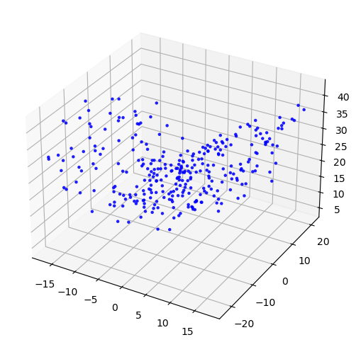
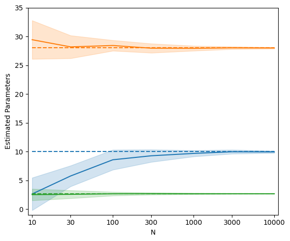
We also infer a \(3\times7\) interaction matrix in a nonlinear gene-regulatory model derived from a published model of B-cell differentiation. These are simulated data, so the true coefficients are available for comparison. Freeness helps interpret why some inferred interactions are less reliable even when the learned system reproduces the sample distribution.

The broader lesson is that reproducing a cloud and recovering a mechanism are different checks. Both deserve attention. A useful reconstruction should report which model parameters the observations constrain and where the ambiguity remains.

What changes when the population is still evolving?

If the distribution changes over time, the stationary balance used above is no longer valid. Time-labeled snapshots contain additional information about that change, even when individual cells cannot be tracked.

For stationary data, the opportunity is already substantial: physical consistency can turn a static population into constraints on dynamical laws. The strength of those constraints depends on the observations and the model assumptions, and DyNoSeD makes that dependence explicit.